Quadrupole Theory Deep Dive

1. Scope and notation

The canonical quadrupole derivation is elegant, but by itself it can leave gaps when you try to explain why one instrument transmits better than another, why a scan line that should work does not, or why source behavior dominates observed performance. This page keeps the derivation explicit and then layers in the practical terms that working instrument scientists care about.

Throughout this page, the quadrupole is treated first as an ideal transverse field with infinitely long rods. That model gives the Mathieu equation and the standard stability diagram. Real instruments are finite, so transmission is a finite-time traversal problem with limited acceptance in transverse phase space and sensitivity to injection conditions.

x, y: Transverse coordinates in the quadrupole field.
r0: Field radius (distance from axis to the ideal hyperbolic electrode surface).
U: DC component on one rod pair (with opposite sign on the orthogonal pair).
V cos(Ωt): RF component (here V is the zero-to-peak amplitude in the stated convention).
Ω: Angular RF drive frequency.
ξ = Ωt / 2: Dimensionless time used to map the equations to Mathieu form.
a, q: Mathieu parameters; signs and scaling depend on voltage convention.
L: Effective filter length (fringing fields make the exact boundary fuzzy).

Many derivations differ by factors of 2 or 4 because of voltage and potential definitions. The physics is unchanged, but the bookkeeping must be internally consistent.

2. Ideal quadrupole field from Laplace's equation

In an ideal quadrupole mass filter, the electrodes produce a transverse potential that satisfies Laplace's equation and has quadrupolar symmetry. Ignoring end effects and axial variation, the scalar potential can be written as a second-order harmonic in x and y.

$$\begin{aligned} \nabla^2 \Phi(x,y,t) &= 0 \\ \Phi(x,y,t) &= \frac{\phi_0(t)}{2r_0^2}(x^2-y^2) \\ \phi_0(t) &= U - V\cos(\Omega t) \end{aligned}$$

This is one common convention. Choosing U + V cos(Omega t) instead flips the sign of q, which is equivalent to a phase shift in the RF drive.

Taking the gradient gives the electric field components:

$$\begin{aligned} E_x &= -\frac{\partial \Phi}{\partial x} = -\frac{\phi_0(t)}{r_0^2}x \\ E_y &= -\frac{\partial \Phi}{\partial y} = +\frac{\phi_0(t)}{r_0^2}y \end{aligned}$$

The symmetry is the key to quadrupole filtering: at a given instant the field focuses one transverse axis while defocusing the other. The alternating field can produce net bounded motion in both axes for selected ions when the operating point falls inside a stability region.

Exact equipotential contours from the ideal quadrupole field

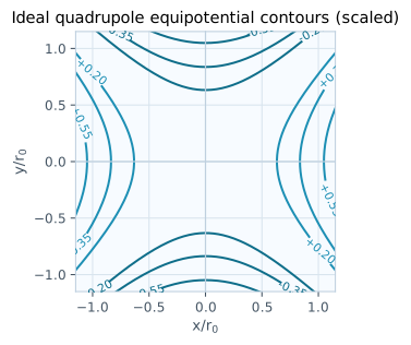
Mathematically generated contour plot of the ideal quadrupole potential in the x-y plane.

These contours are computed from the ideal dimensionless potential proportional to x^2 - y^2, not hand-drawn curves.

Field-vector snapshot from the same potential (exact gradients)

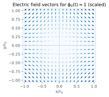
Mathematically generated vector-field plot of the ideal quadrupole electric field at a fixed RF phase.

The arrows are computed from E = -grad(Phi) for a fixed field phase, showing the instantaneous focus/defocus symmetry explicitly.

3. Deriving the Mathieu equation

For an ion of charge +e and mass m, Newton's law gives the transverse equations of motion directly from the field above.

$$\begin{aligned} m\frac{d^2x}{dt^2} &= eE_x = -e\left[\frac{\phi_0(t)}{r_0^2}\right]x \\ m\frac{d^2y}{dt^2} &= eE_y = +e\left[\frac{\phi_0(t)}{r_0^2}\right]y \end{aligned}$$

Substitute phi0(t) = U - V cos(Omega t):

$$\begin{aligned} \frac{d^2x}{dt^2} + \left[\frac{e}{mr_0^2}\right]\left[U - V\cos(\Omega t)\right]x &= 0 \\ \frac{d^2y}{dt^2} - \left[\frac{e}{mr_0^2}\right]\left[U - V\cos(\Omega t)\right]y &= 0 \end{aligned}$$

Introduce dimensionless time xi = Omega t / 2. Since d^2/dt^2 = (Omega^2/4) d^2/dxi^2, multiply through by 4/Omega^2 to obtain:

$$\begin{aligned} \frac{d^2x}{d\xi^2} + \left[\frac{4eU}{mr_0^2\Omega^2} - \frac{4eV}{mr_0^2\Omega^2}\cos(2\xi)\right]x &= 0 \\ \frac{d^2y}{d\xi^2} - \left[\frac{4eU}{mr_0^2\Omega^2} - \frac{4eV}{mr_0^2\Omega^2}\cos(2\xi)\right]y &= 0 \end{aligned}$$

Compare to the canonical Mathieu equation

$$\frac{d^2u}{d\xi^2} + \left[a - 2q\cos(2\xi)\right]u = 0$$

which gives, for this convention:

$$\begin{aligned} a_x &= \frac{4eU}{mr_0^2\Omega^2} \\ q_x &= \frac{2eV}{mr_0^2\Omega^2} \\ a_y &= -a_x \\ q_y &= -q_x \end{aligned}$$

Convention difference	What changes	What does not
Use `U + V cos(Omega t)`	`q` sign flips	Stability physics (phase reference shifts)
Use peak-to-peak RF instead of zero-to-peak RF	`q` scales by 1/2	Shape of stability regions
Different prefactor in `Phi`	`a`, `q` rescale	Physical bounded vs unbounded trajectories

In practice, the dominant source of "wrong equation" arguments is not physics but inconsistent use of electronics voltage calibration (especially RF amplitude reporting) against a design formula written in another convention.

4. Stability regions and scan-line operation

The Mathieu equation has bounded and unbounded solutions depending on the pair (a, q). The set of bounded solutions defines the stability regions. For quadrupole mass filters, the first stability region (the one near the origin) is the one typically used for mass filtering.

Because a and q scale as 1/m for fixed U, V, r0, and Omega, ions of different masses occupy different points along the same scan line. The instrument passes ions whose trajectories are simultaneously stable in both transverse axes over the finite filter length.

Mass filtering mode (RF + DC)

A scan line with fixed U/V is swept in amplitude. Ions cross the apex region of the first stability zone one mass at a time. Narrower effective stability occupancy means higher resolution, but usually lower transmission.

RF-only mode (ion guide behavior)

With U = 0, a = 0 and stability is determined by q. This behaves as a mass-dependent transmission guide with a low-mass cutoff set by the RF amplitude and frequency.

For a quadrupole mass filter, the physically relevant region is the simultaneous stability of the x and y equations. Using the phase-shift argument for the y-equation, the branch limits in the first quadrant can be written with Mathieu characteristic values as:

$$\begin{aligned} x\text{-axis stability: } & a_0(q) \le a \le b_1(q) \\ y\text{-axis stability (mapped): } & -b_1(q) \le a \le -a_0(q) \\ \Rightarrow\; \text{quadrupole mass-filter region: } & 0 \le a \le \min\!\left[-a_0(q),\, b_1(q)\right] \end{aligned}$$

The \"apex\" used in quadrupole scan-line discussions is the maximum-a point of this envelope, which occurs where the two branch limits cross: -a0(q) = b1(q).

$$\begin{aligned} a &= C_a \frac{U}{m} \\ q &= C_q \frac{V}{m} \end{aligned}$$

Here C_a and C_q collect the constants and convention choices (including e, r0, Omega, and RF voltage definition).

In many standard conventions, the apex of the first stability region occurs near (a, q) = (0.237, 0.706). Confirm the convention before reusing published numbers.

Exact first quadrupole mass-filter region with scan lines

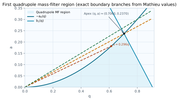
Exact quadrupole mass-filter first stability region plot from Mathieu characteristic values with scan lines overlaid.

This plot is generated from the exact branch functions a0(q) and b1(q) (via SciPy Mathieu characteristic values) and shows real scan lines intersecting the envelope.

Exact branch limits and envelope crossing condition

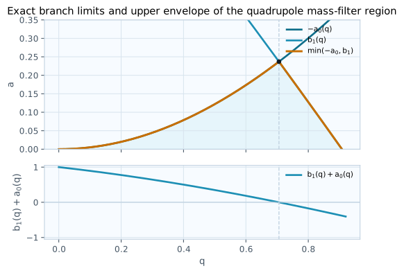
Exact plot of minus a0(q), b1(q), their envelope, and the crossing function b1(q)+a0(q).

The lower panel shows the exact crossing function b1(q) + a0(q); its zero defines the apex where the upper envelope switches branches.

Finite-length consequence that textbooks often postpone

The Mathieu stability map describes infinite-time boundedness. A real mass filter has finite length L, so the experimentally relevant question is: does the ion remain within the mechanical aperture for the time it takes to traverse the rods? This is why acceptance and injection conditions matter so much in practice.

Open interactive stability diagram

5. Secular motion, micromotion, and pseudopotential intuition

In the stable regime (especially for moderate q), the ion trajectory can be viewed as a slow secular oscillation with a superimposed RF micromotion. This decomposition is not exact everywhere, but it is a powerful design and diagnostic intuition tool.

$$\begin{aligned} x(\xi) &\sim A\cos(\beta \xi + \phi)\left[1 - \frac{q}{2}\cos(2\xi) + \cdots \right] \\ \omega_{\mathrm{sec}} &\sim \frac{\beta \Omega}{2} \end{aligned}$$

Here beta is the Mathieu characteristic exponent. Near the origin of the first stability region and for small-to-moderate q, one often uses approximate expressions for beta (their exact form depends on axis and convention). The point is conceptual: the RF field creates rapid modulation on top of a slower envelope.

In RF-only guides, the pseudopotential approximation provides a useful averaged picture of radial confinement. Near the mass-filter apex, however, where high selectivity is obtained by operating close to the stability boundary, pseudopotential intuition becomes less reliable and full trajectory calculations matter more.

Practical translation: pseudopotential thinking is excellent for building intuition about guides and transport optics, but high-resolution mass filtering performance is usually limited by boundary effects, finite transit time, fringing fields, and source-beam mismatch rather than by the simple averaged potential picture alone.

6. Phase-space acceptance and finite-length transmission

For a finite quadrupole, transmission is not just a yes/no function of (a, q). It is a phase-space problem. An ion entering the filter is described by position and angle (or transverse momentum) in both axes, plus axial velocity, kinetic-energy spread, and RF phase at injection. The filter transmits only the subset of those initial conditions that remain within the rod aperture for the traversal time.

This subset is the acceptance. In the most practical lab sense, people talk about a quadrupole's "acceptance" as if it were a single number, but in reality it is a multidimensional region that depends on operating point, RF phase, energy spread, and the end-field geometry.

Transverse phase space

At minimum, consider (x, x', y, y'), where x' = dx/dz and y' = dy/dz represent angles relative to the axis. Acceptance is the region in this space that survives the filter.

Why RF phase matters

The quadrupole field is time-dependent. Two ions with identical spatial coordinates but different injection RF phase can experience different early-cycle kicks and therefore different outcomes.

Phase-space acceptance and beam ellipse (computed)

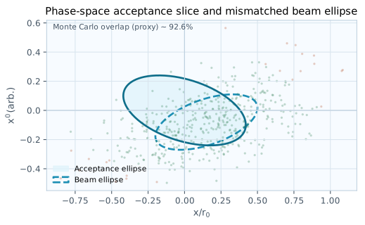
Mathematically generated phase-space plot showing a quadrupole acceptance ellipse and a mismatched source beam ellipse with sampled points.

This is a quantitative phase-space construction (with a Monte Carlo overlap proxy), illustrating why transmission depends on distribution overlap rather than source current alone.

Finite-length trajectories from direct numerical integration

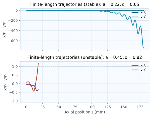
Numerically integrated stable and unstable quadrupole trajectories versus axial position for finite rod length.

These trajectories are obtained by directly integrating the canonical Mathieu-form equations for chosen (a,q) pairs over a finite number of RF cycles.

What shrinks or distorts acceptance in practice

Operating closer to the stability boundary for higher resolution.
Fringing fields at the filter entrance and exit (non-ideal axial variation of the field).
Energy spread and axial velocity spread (different transit times and RF phase histories).
Source-beam mismatch (beam emittance larger than or poorly aligned with acceptance).
Rod misalignment, RF imbalance, and field distortion from contamination or tolerances.
Space-charge effects at high ion current (beam self-fields and broadened distributions).

In other words, a quadrupole mass filter is not just a point on the Mathieu diagram. It is a dynamic acceptance system that must be matched to the source and transport optics.

7. Emittance vs "emissivity" (terminology and source matching)

In ion optics, the technically correct term for the beam's occupied phase-space area is emittance, not emissivity. In practice, people sometimes say "source emissivity" when they mean how broad or well-collimated the emitted ion beam is, or how much usable current the source produces. It is worth separating these ideas because they affect quadrupole performance in different ways.

Beam emittance (ion optics term)

Describes the position-angle spread of the beam (for example in x-x' and y-y' space). Large emittance or poor matching reduces the fraction of ions that fit within quadrupole acceptance.

Source output / brightness

Total ion current alone is not enough. What matters for transmission is current per unit emittance (brightness) and how that distribution is matched to the quadrupole entrance optics and operating point.

A common failure mode in method optimization is to maximize source current while ignoring the angular spread or energy spread of the beam. The measured current at the source or prefilter can increase while quadrupole transmission, stability near the scan apex, and spectral quality become worse because the beam no longer fits the acceptance.

Source parameters that strongly influence quadrupole transmission via emittance and energy spread

Extraction field geometry and voltages (beam divergence and initial phase-space ellipse orientation).
Source pressure / collisionality (cooling can reduce emittance; excessive collisions can broaden energy spread or cause clustering).
Plume geometry, capillary alignment, skimmer alignment, and source contamination.
Desolvation/thermal conditions in atmospheric-pressure interfaces (changes droplet/cluster survival and ion energy spread).
Space charge at high source currents (self-field expansion and nonlinear transport effects).

Quadrupole transmission ~= overlap(source distribution, quadrupole acceptance)

This overlap depends on:
  (x, x', y, y') distribution
  energy spread and axial velocity spread
  injection RF phase distribution
  end-field geometry and alignment

If you meant "ion source emissivity" in the sense of ion-emission efficiency or source output quality, the most quadrupole-relevant quantities are beam emittance, energy spread, and stability of those quantities over time.

8. Thermal emissivity of source and quadrupole rods

Thermal emissivity (radiative emissivity) is a different concept from beam emittance, but it can still matter in quadrupole systems. The ideal Mathieu derivation assumes perfect geometry and prescribed voltages; it does not model temperature, outgassing, adsorption/desorption, or surface-condition drift. Real instruments do.

Why source thermal emissivity can matter

Source wall temperature affects desorption, clustering, and contamination release/adsorption behavior.
Radiative heat balance influences warm-up time and thermal stability of nearby optics and insulators.
Thermal state can change outgassing load, which affects pressure and therefore collisional transport and background.
In hot sources, temperature-driven chemistry and ion-molecule processes can alter the distribution entering the quadrupole.

Why quadrupole rod thermal emissivity can matter (indirectly)

Rod emissivity usually does not enter the equations of motion directly, but it influences the rods' thermal equilibrium and therefore several second-order effects that become operationally important.

Warm-up behavior and thermal gradients (which affect dimensional stability and alignment at a small but nonzero level).
Surface contamination adsorption/desorption cycles, which alter patch potentials and field quality more directly than emissivity itself.
Outgassing and recovery after contamination or venting, via temperature-dependent surface processes.
Temperature of rod supports and nearby dielectrics, which can affect leakage, charging, and stability.

Category	Examples	Effect on quadrupole behavior
Direct field-defining parameters	`U`, `V`, `Omega`, `r0`, geometry symmetry	Set `a`, `q`, stability mapping, and ideal filtering behavior.
Transport and matching parameters	Source emittance, energy spread, alignment, end fields	Set effective acceptance overlap and therefore transmission/resolution in practice.
Thermal / surface parameters	Source/rod thermal emissivity, contamination films, outgassing state	Indirectly shift stability, noise, and reproducibility through temperature and surface condition.

In many instruments, surface cleanliness and RF phase/amplitude balance dominate performance changes before thermal emissivity does. Emissivity matters primarily because it helps set the temperature and surface history that those more direct effects depend on.

9. Non-ideal fields and engineering realities

The ideal quadrupole is a foundational model, but performance is often limited by deviations from that model. Good quadrupole engineering is about controlling which non-idealities matter at the required resolution and sensitivity.

Common non-idealities with large practical impact

Electrode geometry approximation: circular rods approximate hyperbolic electrodes only for a chosen ratio of rod radius to field radius. Geometry errors introduce higher multipole components.
Rod alignment and spacing tolerances: asymmetry shifts stability boundaries, broadens peaks, and degrades abundance sensitivity.
RF amplitude and phase imbalance: imperfect drive symmetry changes the effective field and can reduce transmission or distort mass calibration behavior.
Fringing fields at the ends: ions see non-ideal entry/exit fields, so finite-length transmission differs from infinite-length predictions.
Electronic waveform purity: harmonic content and noise produce field perturbations and can widen peaks or shift apparent operating points.
Space charge: high ion current can broaden the beam distribution and alter trajectories, especially upstream of the filter.
Contamination and patch potentials: surface films can distort local fields and worsen long-term reproducibility.

Textbook-limited thinking

"The point is in the stability region, so transmission should be high." This misses finite length, injection phase, emittance mismatch, and end-field effects.

Instrument-limited thinking

"The rods are dirty, so the math is useless." Also wrong. The ideal model still defines the baseline behavior; the engineering problem is quantifying deviations from it.

10. Practical tuning and troubleshooting implications

The value of quadrupole theory is not only in deriving a and q, but in making better decisions when performance drifts. The checklist below translates the theory into an engineering workflow.

Start with the field-defining parameters. Verify RF amplitude calibration, frequency, DC/RF ratio, and scan electronics assumptions (including voltage convention).
Confirm finite-length and matching conditions. Evaluate source alignment, extraction optics, prefilter settings, and signs of emittance/acceptance mismatch.
Check energy spread and stability of the injected beam. A beam with high current but poor energy/angle distribution can collapse transmission near higher-resolution settings.
Inspect end-field and contamination clues. Look for changes after venting, source cleaning, rod cleaning, or maintenance; end effects and patch potentials often dominate unexplained behavior.
Trend performance, not just single runs. Mass accuracy, transmission, background, and peak-shape trends reveal thermal and surface-history effects that a single tune snapshot hides.
Write down the convention. Include whether RF amplitudes are zero-to-peak or peak-to-peak and which parameter formulas you used. This prevents future factor-of-two confusion.

Back to tutorials Method development section Troubleshooting section

11. Suggested references and next study topics

If you want to go deeper than this page, the next step is to study full Mathieu stability analysis, Floquet theory for periodic systems, trajectory simulation of finite-length quadrupoles with fringing fields, and ion-optical beam matching (Twiss-parameter style descriptions and emittance transport).

Classic quadrupole mass spectrometry texts (theory + instrument design chapters).
Mathieu-function and Floquet-theory references for periodic differential equations.
Ion optics references on beam emittance, brightness, and acceptance matching.
Instrument papers and application notes on prefilters, rod geometry tolerances, and abundance sensitivity.
Vacuum/surface-science references for outgassing, contamination, and temperature-driven recovery behavior.

A useful exercise is to take one quadrupole method in your lab, write down its implicit assumptions (source conditions, beam stability, scan settings, acceptable drift), and map those assumptions onto the categories in this article: field-defining, transport/matching, and thermal/surface-state factors.